Reproducing Analysis of Large Single-Cell RNA Seq Datasets

Introduction

Since the first commercial Single-cell RNA sequencing (scRNA-seq) platform became available in 2014, the size of single cell datasets has expanded significantly (Fig 1A). What was once prohibitively expensive – sequencing hundreds of thousands of cells for an experiment – is now common practice (Fig 1A, B).

While hardware and chemistry-based practices have evolved to enable sequencing increasingly large samples, other downstream barriers still exist to analyzing large single cell datasets. First, the scale of scRNA-seq data necessitates substantial computational resources for data storage, processing, and analysis. Certain tasks, such as batch effect correction and batch integration, are particularly resource-intensive and virtually impossible without access to scalable computational solutions. Second, bioinformatics analysis tools for scRNA-seq data often have steep learning curves and may require advanced computational skills.

Here, we demonstrate how g.nome offers a scalable, no code, transparent solution for analyzing large datasets by reproducing the analysis of Wu et al (2022).  We highlight g.nome’s data filtering, batch integration and batch effect correction, and clustering capabilities on a dataset of 26 samples and 100,064 cells.

Objectives

• Reproduce Analysis of Public Data: We demonstrate how to use g.nome to reproduce analysis of a public dataset, and compare results generated on g.nome to those published by Wu et al.
  
  
• Demonstrate Transparency: We outline the workflows used for analysis, demonstrating how g.nome is designed for transparent and reproducible analysis.
  
  
• Utilize Advanced Bioinformatics Without Code: Employ the g.nome® platform for in-depth scRNA-seq analysis.
  
  
• Integration & Batch Effect Correction: When combining scRNA-seq datasets from different experiments, sources, or conditions, batch effects—systematic non-biological differences between datasets—can confound analysis. Here, we compare data before and after batch effect correction to demonstrate how computational methods that can accurately integrate data across batches ensure valid biological interpretations.
  

Methodology

Counts data in MEX format was obtained from Gene Expression Omnibus with the serial number GSE176078. 

Analysis was performed on g.nome following the methods outlined in Wu et al.’s methods section and supplementary note. 

Filtering, Normalization, and Data Reduction

Filtering was done using g.nome’s Seurat-subset tool, which enables filtering by number of UMIs observed per cell, number of genes observed per cell, mitochondrial DNA, and complexity (ratio of genes to UMIs).  

Seurat-subset:

• Min Number of UMIs = 250
• Min Number of Genes = 200
• Max % Mitochondrial Genes = 20

Data normalization was performed with Seurat-normalization using default parameters (“LogNormalize” normalization method, scale factor of 1000). For the merged analysis without batch effect correction, all 26 samples were merged post-normalization with Seurat-merge. Samples were reduced to the top 2000 most variably expressed genes using Seurat-findvariablefeatures. 

Integration and Batch Effect Correction

When combining scRNA-seq datasets from different experiments, sources, or conditions, batch effects—systematic non-biological differences between datasets—can confound analysis. Computational methods that can accurately integrate and normalize data across batches are necessary to ensure valid biological interpretations.

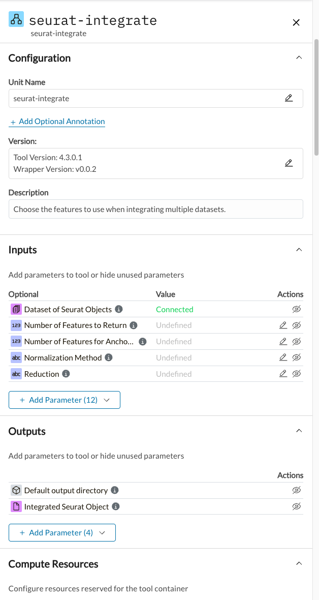
For the integrated analyses, a dataset of 26 Seurat objects was passed to Seurat-integrate, which uses Seurat-FindIntegrationAnchors and Seurat-IntegrateData. Integration can often be impossible or painfully slow without an HPC. On g.nome tools can be allocated up to 256 GB of RAM, enabling computationally intensive steps such as data integration.

Additionally, while Wu et al. used Seurat’s default Canonical Correlation Analysis (CCA) reduction method, a more conservative alternative method called Reciprocal PCA (RPCA) can also be used on g.nome for integrating large datasets. 

• CCA is better for samples with conserved cell types, but experimental or disease conditions may introduce strong expression shifts. 
• RPCA is significantly faster and more conservative; best suited for large datasets, datasets originating from the same platform, and datasets with inconsistent cell types across samples.

For more information on CCA vs. RPCA Integration, refer to the Seurat vignette here.

Seurat-integrate

• Number of Features for Anchor Finding = 2000
• Weighting Dimensions = 30
• Algorithm = Canonical Correlation Analysis (CCA)

Dimensionality Reduction & Clustering

Expression levels across cells were standardized using Seurat-scaledata with default settings. Linear dimensionality reduction was performed using Seurat-runpca and the first 100 principal components were returned. 

Per the authors’ instructions, for the integrated data, clustering was performed using Seurat-findneighbors with 30 dimensions and Seurat-findclusters with a resolution of 0.8. Seurat-dimplot was used to perform UMAP reduction with 30 dimensions.  

For the merged data without batch effect correction, clustering was performed using Seurat-findneighbors with 100 principal components and Seurat-findclusters with a resolution of 0.8. Seurat-dimplot was used to perform UMAP reduction with 100 principal components.   

Results

Key usage statistics:

Analysis with data integration and batch effect correction:

• Analysis Time: 5h 57 min
• Quantity of Data Processed: 2.06 GB (26 samples, 100,064 cells)

Analysis on merged data, without batch effect correction:

• Analysis Time: 3h, 6 min
• Quantity of Data Processed: 2.06 GB (26 samples, 100,064 cells)

Quality Control 

We verified that the filtered data used in downstream analysis was identical to Wu et al’s by visualizing distributions of two quality metrics: number of UMIs per cell and number of genes per cell.

Clustering – Merged data without batch effect correction

We reproduced Wu et al. UMAP visualization of the merged dataset without batch effect correction. 
UMAP plots enable visual representation of high-dimensional single cell data in two-dimensional space. Here, thousands of variables (genes) are reduced to two embeddings (UMAP_1, UMAP_2) which represent a combination of the genes which demonstrated the highest level of variance across cells. Each point represents a cell. Points that group closely together to form clusters have similar expression profiles, which can indicate cell type, cell state, or other biological groupings.

Wu’s Extended Fig 1e-f are shown on the left, and g.nome’s recreations on the right. Both figures represent 71,220 Immune and Stromal Cells (Cancer and Normal Epithelial Cells removed). The top row shows the cells colored by sample ID, and the bottom row shows the cell colored by major cell type. Cell type annotations were obtained from the  provided metadata. 

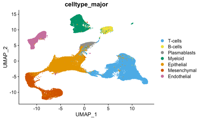
Clustering – Integrated data with batch effect correction
Integrated dataset of all 100,064 Cells from 26 patients

We reproduced Wu et al. UMAP visualization of the integrated dataset with batch effect correction. Both figures represent 100,064 cells. Cell types were obtained using the provided metadata. 

It is important to note that UMAP is a stochastic algorithm, which means that different runs with the same parameters may produce slightly different results, although there are certain strategies which can be used to evaluate whether two UMAP projections effectively capture the same underlying meaning. Here the overall pattern and distribution of points is very similar. Exact positions and orientations may differ, but clusters appear in roughly the same areas. Shapes of and distances between clusters differ slightly, but relative positions and separation distances of clusters are similar. It's also useful to remember that UMAP, by design, focuses more on preserving local neighborhood structures than global distances, so evaluation methods should prioritize these aspects.

Conclusion

In conclusion, g.nome emerges as an indispensable tool in the realm of single-cell analysis, empowering researchers to unravel the intricacies of cellular composition with unprecedented accuracy and efficiency. By leveraging advanced bioinformatics methodologies and comprehensive reference datasets, g.nome catalyzes groundbreaking discoveries, propelling the field of cellular biology into new frontiers of understanding and therapeutic innovation.