Webinar: Bulk RNA-Seq Analysis for Biomarker Discovery

 

 

Hannah Schuyler graduated from The University of Texas and spent the beginning of her career focused on using digital analytics to inform a marketing strategy for pharmaceutical, biotech, and medical device clients. She has spent the last few years working with clients to help them identify data analysis solutions for NGS and genomic data.

 

Speaker

 

---

 

Transcript

Hannah Schuyler:

Hi, everyone, and welcome to today's webinar: Bulk RNA Sequencing for Biomarker Discovery. My name is Hannah Schuyler, I'm a Director of Business Development here at Almaden Genomics, and joining us today is Mark Kunitomi, who is one of the co-founders here at Almaden and also our Chief Science Officer.

Today, what we'll be discussing is first we will be giving you guys an introduction to Almaden Genomics and who we are, really highlighting our end-to-end solution and the importance of being able to process your raw sequencing files all the way to tertiary analysis. Mark will then give you an overview of the dataset that we'll be analyzing today, which is focused on colorectal cancer. Then he will give a demo of how you can actually use g.nome to process your data files and interpret your data with all of the different interactive visualizations that we have. And then lastly, we'll leave time for Q&A.

When it comes to analyzing data, there are many complexities that make it very challenging to analyze these data sets. The first thing is really around the fact that there's massive amounts of data across different workstreams and teams—there’s difficulty when it comes to managing this data in one secure place, and there's often a communication gap between both the biologists and the bioinformaticians, it's a very iterative process. When it comes to analyzing the data, the biologists often relying on the bioinformatician, and it's not always a streamlined. This ultimately will slow down the time for analysis and discovery. There's also a need for transparency and organizing organizational systems to track and reproduce methods for future experiments.

With all of that being said, here at Almaden Genomics, we're looking to provide an end-to-end solution for our customers. And so that first step really begins with the data and bringing that into the software. Whether that's your own in-house sequencing data that you're working with or public datasets that you're looking to analyze, all of that data can be brought in to g.nome. Then, the next step is around data processing—you can use g.nome to start with our prebuilt workflows, modify them, or build a pipeline from scratch. The next step is then focused on the tertiary analysis and making sense of the data—g.nome produces some visualizations to help with interpretation. We have heatmaps, volcano plots, and all sorts of interactive visualizations and reports that you can share with team members across the organization.

Then there's the service component, which is where we can really help with many steps along the way, like bringing in data, curating it, or harmonizing those datasets that we've identified; and then of course the bioinformatics support, such as building pipelines or helping from a data analysis standpoint.

Today's webinar is going to focus on g.nome and how you can actually use that to process your bulk RNA sequencing data. I think one of the unique aspects of this software is that it can meet you at your computational skill level, giving you access to multiple different interfaces and really allowing both the biologists and bioinformaticians to interface with the data. You can also scale your analysis with our high-performance cloud environment, ultimately allowing you to increase the amount of data that can be processed. There's also a reliable and auditable environment allowing you to track changes to a workflow and easily reproduce those experiments moving forward.

As I mentioned, this software has multiple different interfaces depending on your bioinformatics skill level. We have a guided workflow option that is essentially a prompted form that allows you to start with a prebuilt workflow, it does not require code, and you can easily process your data—this is a great way for biologists that are doing routine analysis to process their data in a few hours and generate meaningful results. For the researcher who wants to customize the workflow and really wants to get under the hood in terms of what's being done with the steps and the tools, we have what's called our Canvas Builder. This is where you have the ability to modify any workflow, you can adjust parameters, swap out tools, and it's all done with our easy-to-use GUI. You also have the ability to analyze data from any starting spot, whether it's raw or processed data, it really gives you full flexibility when it comes to processing your data.

You can also do tertiary analysis on the software. Some important analysis that researchers are doing often are gene set enrichment analysis (GSEA), comparing gene signatures, and exploring drug connectivity, these are all different types of reports that can be done within the software.

With that, I'm going to pass it over to Mark to walk through the research objectives that we'll be talking through specifically with this public data set, looking at colorectal cancer.

Mark Kunitomi:

Thanks so much Hannah. For today's webinar, what we're going to be doing is accessing some publicly available RNA sequencing data sets and analyzing them using the g.nome platform. The g.nome platform makes it really easy to be able to analyze these sorts of datasets without using code. I myself started as a wet lab biologist and was forced to learn how to become a bioinformatician because that's all that was available at the time.

The g.nome platform really allows you to do this purely with our guided workflows and our graphical user interface. So for today, well, we're going to start with is we're going to access some data from the Sequence Read Archive (SRA) and pull some accessions for these publicly available datasets and upload those into g.nome using those accessions. With one of our guided workflows, we're going to download all of that data into the g.nome system, which resides on the cloud.

Once we have all of that data, we're going to start to analyze that using g.nome systems. Once we've gotten a bit into that analysis, we're going to want to verify the quality of those datasets because after all, they are publicly available and they're coming from various different labs or using various different processes. And lastly, once we've gone through that, we can interpret the results that we get using the visualizations that are automatically created from g.nome.

Today we're going to be looking at a dataset or a set of datasets from colorectal cancer (CRC). Colorectal cancer is really a pressing health issue due to its high incidence and mortality rates. It is one of the leading cause of cancer related deaths, and its incidence is increasing due to aging and lifestyle factors. Studying colorectal cancer is really crucial because of the profound genetic impact on its progression—mutations that occur in tumor suppressor genes or oncogenes drive colorectal cancer, but also alter gene expression. So, understanding these transcriptomic changes or changes in RNA expression is really essential for uncovering the underlying mechanisms for colorectal cancer, as well as its progression and for identifying biomarkers which are invaluable for early diagnosis, accurate prognosis and predicting treatment responses.

Today we're going to be taking a look at a paper that came out on Scientific Reports. One of the really cool things about this paper, at least to me, is that they didn't do any of the RNA sequencing in-house. They were able to leverage publicly available datasets, integrate them together and analyze them in order to look for prognostic biomarkers.

And once they found a list of candidates, they followed those up through qPCR validation and found a couple of genes that they think of as being good as prognostic biomarkers. Taking a closer look at the data that they pulled together, they brought together four different data sets that were available on SRA, do these are publicly available datasets brought there from several different labs, and each of them contains several colorectal tumor tissue samples as well as adjacent normal tissues.

One of the beauties of being able to bring together multiple different datasets that come from different labs is first off, it's going to enhance your statistical power. The more samples that you have, the more confidence you can have in the genes that you find that are upregulated and downregulated or pathways, etc. The other thing that I think is really valuable when you're bringing data from disparate sources is that you get cross-study validation—those biomarkers that you get out of an analysis are coming from multiple different labs, so when you get results that are consistent across labs, across studies, across techniques, I think that gives you a lot more confidence that these are going to be recognizable in the clinic or in your own lab.

In order to replicate this study and be able to do further downstream analysis, the first thing that we're going to do is import this RNA sequencing data, based on the accessions that are available from this paper. That paper has a data availability section, so I’m just grabbing those file projects, using those in order to run a guided workflow on g.nome to pull in that data very rapidly and easily, even though it's going to be, you know, hundreds of gigabytes of data, we're going to be able to bring that into the g.nome quite rapidly.

Second thing that's going to be really important is to do quality control, both on the sequence itself as well as the alignments that we're going to get, how we relate it to the human transcriptome. Lastly, we're going to look at differential expression analysis to see between those tumors and normal tissues what genes are upregulated or downregulated, what pathways, and gene sets as well.

For the first part of this analysis, we're not actually going to show it to you, but essentially I just went into this paper, grabbed the four bio projects that is listed in the data availability section and from there went to SRA to grab those accessions. We're going to start our demo in just a second using those accessions and uploading them into g.nome.

Once you've logged into g.nome, it's going to take you to our “Projects” page. g.nome is a web based SAS application that sits on AWS so you have access to it basically anywhere that you have a connection to the internet. And because it sits on AWS, but we do all of the management of that infrastructure, you really don't need to worry about where the data is stored or how the computation is going to be performed. All of that is going to occur on the cloud in a cloud elastic nature, which is very scalable without you needing to manage any of that infrastructure.

On g.nome, we use a project based organization for how we run analysis. We have a workspace here that's going to be shared amongst various team members. We usually see that that our users have a single workspace for a particular lab, and projects themselves can be used in various different ways.

One, you can just create a project, bring in your data, bring in a premade workflow, run the analysis, and get on to interpretation. You can also use a project to bring in some of our pre-made workflows and make customizations, if you need to make those types of customizations. Or, you can use them to build a workflow from scratch using our workflow builder. For today, because we don't have the time to run a full analysis end to end, because some of these analyses are going to take 10 minutes, some of them are going to take 5 to 10 hours, we're going to do this in a bit of a cooking show style where we can go through and set up each one of these workflows as well but then look at one that's already been completed.

When we open up a project, we're going to start on the summary page that's going to include who created it, and you can search for projects based on the user. I created this project, it contains a description if the creator was responsible enough to do that, and then a summary of the workflows that have been brought in, the tools that are brought in, and of course the cost that's been incurred on this project.

So far I've been doing quite a bit of testing on this and we can see that there are several workflows that have already been run and I've brought in quite a bit of data centers, 821 gigs that was brought into this project as well as the associated cost. Looking at the top of this project, we can see that it's separated by tabs into the various functions that you're going to want to perform.

What's in a project? We have our “Data” tab, “Tools” tab, “Workflows” tab, and “Runs” tab, which I'm going to get into next few minutes. One of the first things that we're going to want to do is bring data in, and there's a few different ways that you can bring data into g.nome. First and foremost, you can bring any data that you have on your local computer. In our top right, we can go to local files from there you can just drag and drop data in in order to upload. These could be very small files like the files that I'm uploading right now, which will have the accessions that we're going to need to download the data as well as some metadata that we pulled off of this.

You can also do this for very large files. We have users who are bringing in their FASTQ files which themselves can be several gigs to ten gigs to like 30 gigs apiece. I'm going to click upload and it's going to have this swing up or down here that I can take a look at in order to check on progress for these files. They're really small, so they complete almost immediately.

In addition to being able to bring in data from your local computer, you can also hook up S3 buckets to our system. If you have a large amount of data that's already on the cloud, you can go through a process of hooking up that S3 bucket and then you can click over here into items from S3 and then you can grab any data that may be associated. We also provide reference data or commonly used genomes and references, as well as test data for all of our tools and our workflows that you can bring in.

And the last way that you can bring in data is to grab publicly available data. For that, we're going to use one of our premade workflows. But before I get into that, I'm going to go and view this accession file, in order to grab all of those accessions that I'm going to need in order to run that workflow, and I'm just going to copy those into my clipboard.

The next thing I'm going to do is go to the workflow sections of this project. I've already imported several workflows and made a workflow within this for our canvas workflows, but we also have our guided workflows, which is what we're going to be using for pulling all of this publicly available data.

So I'm going to click over from the canvas workflows to our guided workflows. g.nome has the ability to run Nextflow code as well as Nextflow pipelines, and we've already brought in several. I'm going to click run for this fetch NGS pipeline. First thing that I'm going to do is it label that run and it starts off with an auto generated name just using an adjective and a famous biologist, but we can also add any customization that we want. So I'm just going to put the dataset that we're doing.

I'll click next from here. I'm going to input those accessions, so that's why I copied them previously. I'm just going to paste them in. As soon as you've pasted these in these accessions in, it's going to do some error checking under the hood. And so if you were to put in a mix of accessions, which is not allowed by this particular pipeline like using SRR and DRR accessions, it's going to immediately tell you that you have these mixed accession types, and it's not going to allow you to go forward.

In addition, if you provide something that's an unknown accession because there's something that's malformed or there was a problem in the copy paste, it'll also throw you a warning telling you that there's an unknown accession and have you check it out before you proceed to the next step.

Now that I have my list of 34 datasets, we can go on to some additional parameters. For this pipeline, you can actually bring in the data in several different ways using FTP, Aspera, or SRA tools. FTP is the default, and it's what we're going to use for today's run. We also have the ability to access the advanced parameters for this workflow. And so if you wanted to be able to look at some of the CPU or memory that's being assigned to these jobs or some additional input or output options, those are advanced parameters for an advanced user who knows exactly what they want to do, that they can choose and bring those onto the workflow and make selections. Then I'm going to click next.

Lastly, it's just going to give us an opportunity to review and launch our job. We know what workflow that we're running, we have the parameters that are going to be listed, the accessions that are part of this, as well as the run label. With that, we're going to click launch. And so on the back end, what's happening is that this is being launched in AWS in the cloud, in a cloud elastic nature.

So each one of the steps of this job is being sent off as an individual module, which is self-contained, and that's going to happen with as much parallelism as possible. So this step of downloading a large amount of data, we're talking hundreds of gigs of data. It's going to take somewhere on the order of 15 minutes to an hour or two.

It sometimes really depends on how fast the service that we're receiving the data is. And so depending on the load NCBI itself is experiencing, it could take as short as this previous run, which took only 12 minutes to bring in this large amount of data, but sometimes a few hours, again, depending on that load on the other side.

When we click into a run as it started, it's going to immediately take us to the tasks and all of the tasks that are being or going to be run. For this, we're going to have a large number of tasks because essentially what's happening is it's identifying each one of these files that's going to be downloaded and then creating a task for each one of these accessions so that it can be downloaded. And we have several of these that are waiting to be kicked off.

In addition, we also get the logs for this run, and then as they're generated, we'll get parameters. So let's take a look at a run that's already been completed. And now that it's completed, it's going to take us to our outputs. And these are the outputs that are generated by fetch NGS. First and foremost, we have our beautiful, beautiful FASTQ files. This is all of the data that was brought in during this process. But in addition to that, will also receive metadata for those files, pipeline info and then sample sheets that are created in the pipeline info can be pretty informative.

These are HTML reports that are generated from the pipeline that are going to include things like how long it took to run each step, what the CPU usage was. Again, these may be a little bit too nerdy for all users, but they can be really important. So take a look at how long things are taking in terms of execution time, where there may be bottlenecks in the system, what's using the majority of the resources. All of these things are available to the user whether or not you choose or need to use them.

Now that we have all of our data, we're going to want to start by running our RNA-seq pipeline. We again have a guided workflow that makes it very easy to be able to initiate this run. I'm going to go over to our guided workflows and we're going to select our bulk RNA-seq pipeline, click run guided workflow, and it's going to give us one of our randomly generated names. I'm just going to add some additional information.

For this workflow, the first thing we're going to need to do is be able to select that data that we brought in previously. We're going to go to our “All Runs” folder that sits in our “Data” tab and we're going to select the workflow that we previously ran in order to bring this in our questioning. There we're going to click into the data folder and then go to those FASTQs files. We have a large amount of data since we brought in 34 samples, we're going to have two times that amount of data in FASTQ files because all of this is paired. One thing I'm going to do is use the search functionality to filter the data to just FASTQ files, and then I'm going to select all of this data for us to analyze within this pipeline.

Once we've selected all of that data, it's going to go through a few steps of validation. We're going to be looking to see does each sample have forward and reverse reads? Do they have the proper extensions and are they properly paired? All of this is done automatically by the system, and as a user, really all you have to do is verify that there's nothing wrong—if there's a sample that you didn't want to include in the analysis, that's something where you can delete a row by going to this actions column and clicking on it If there's a pairing that you believe to be incorrect, you can come in here and then filter to where you think the correct file would be and then select it.

However, the system sees that again, for something that's incompatible, like in this case you've used the same file for forward and reverse reads. Now that we've verified all of our data has been selected correctly, we're going to go on to the next step, which is to group our samples. So ultimately what we want to do is differential expression. We want to compare two groups, our normal tissues compared to our tumor tissues. In order to do that, we need to define which group each sample is part of.

The first thing that I want to do is go to this group list and override the name from control. I'm going to call this the normal group or normal tissues. Then I go from experimental and change it to tumor when it comes up here to our control group and make sure that that's normal, since that will be comparing to the tumors to.

And then we can go through and manually select which group each of these samples should be. Now, when you have a large amount of data, that's a case where you're going to want to have brought in a sample sheet or a sample metadata file. We did that in one of our first steps in our data upload, so I already have a metadata file that's defined for each of these samples, what group they should be in.

And so this is really useful when you have something like 34 samples and you don't want to manually click through each step. Now that we defined our groups to be compared, we go to the next step, where we need to select our reference genome. So this is going to be human data, so we're going to be selecting good old GRCh38.

But if you're working with mouse data, we also have GRCm39, and if you like to use GRCh37 for comparison purposes, that's available as well. And if none of these genomes works for you, you can bring in custom reference data. So if you're working with a non model organism or you have a particular custom genome that you want to be able to utilize, you can click over here, select past a file, select digital files for that and use a custom reference.

But for our purposes, today, GRCh38 is great. Next, that's going to ask us for our recount method. We offer two for this pipeline: feature counts and string time. Feature counts is our default option and this will also work for today. Lastly, we're going to have some of our optional parameters. Our organism is set as human since we’re working on human data, and we can change our default p-value threshold and log-fold change threshold.

But I'm not going to change any of those for today's analysis. With that, I'll click next and then we can go to this review and launch. Ensure that all of this information makes sense in terms of the analysis you want to do and, and then you click launch. This is going to initiate our run. And again, this is something where we can click it into and observe all of the tasks as they're being performed.

Each one of these steps, again, is fully modular and run in the cloud, so for every step that can be parallelized, it will be run in parallel. So we're starting with some RNA sequencing and alignment, and each of these steps is running for each of these samples in parallel, which really speeds up the process, but also performs these analyzes in batch, which is cost effective.

Again, we'll have access to all of the log files as well as the parameters used in order to initiate this run and then outputs as they come along. Because there is a large amount of data for this dataset, this analysis took about seven out just under 7 hours previously. I don't think we're willing to wait that for this webinar, so we’ll just click in to our pre analyzed sample. So once this once run has been completed, it's going to start off by sending us to the outputs and we can see all of the outputs that are produced for this bulk RNA-seq analysis with differential expression. We're going to have our bulk RNA-seq report that is generated as a custom report as well as our quality control data, gene set enrichment data, pathway analysis, as well as some of the raw data.

If you want to be able to analyze the gene count data yourself, or if you have a data scientist that you collaborate with, you may want to take a look at the data.

The first thing that we're going to want to do when we look at the output of this analysis is immediately do some quality control. We grabbed all of this data that came from various different public sources. We want to make sure that it's all of reasonable quality to put into our analysis. What we’re going to do is go to this MultiQC section and take a look at our MultiQC report. So the nice thing is on g.nome you can immediately open these h HTML reports on platforms, though you can also download these to your local computer and send them off to your colleagues as needed if they don't have access to the g.nome or just prefer to receive it in an email.

MultiQC is a really powerful tool that will allow us to look at not only the sequence quality content, but also the alignments to the human and their quality. A nice aspect of this is they also include a tutorial video, so if anything doesn't make sense, you can go and watch their video or read their documentation and it's embedded into this HTML file.

The first thing that I like to take a look at when I'm at QC from from publicly pulled data or even my own are these general statistics. That's going to be broken up into the alignment stats on the left here and then some of the sequencing stats over here on the right. One thing that I think is really interesting to point out about this dataset, because it came from different places and they use different kits and different techniques in order to generate this RNA-seq data, is that you can immediately see that the red lines between these samples are very different.

This sample 507 has a read length of 150 base pairs, whereas this next one has 100 base pairs, and we see ones that are down at 76 base pairs. So we have a very heterogeneous dataset, which I would suppose we expect based on the fact that it's four different experiments that have been pulled together. We also can look at the percent of those reads that have been aligned and we're seeing quite good percentage aligned, which is nice to see. We're going to want to see over 70% of those reads at least aligning to the genome. Then we also have the ability to look at uniquely aligned reads. Again, we're going to see some differences between some of our different samples. Some of them have more duplication and less uniquely aligned and others have a greater amount.

That kind of leads us into our next part of looking at QC, which is the alignment scores. One thing that really jumps out to me when I take a look at this is that we really have three groups of data: one which is large amounts of reads, having somewhere on the order of 30 to 50 million reads; we have a group of kind of a medium amount of reads, somewhere between, let's say 20 and 30; and then we have data that has a lot less reads, somewhere between five and 10 million. So again, bringing in disparate data means that that's going to be quite heterogeneous and that's something to really look at later, which we'll kind of take a look at when we look at the picture.

Another really important aspect is to look at the sequencing quality. We know that the data is very different, but that doesn't necessarily mean some of that data is good and some of that data is bad. We can see from looking at the sequence quality histograms that although there are different read lengths and different amounts of duplications, all of the sequencing data itself is of quite high quality that exists on kind of a per base content.

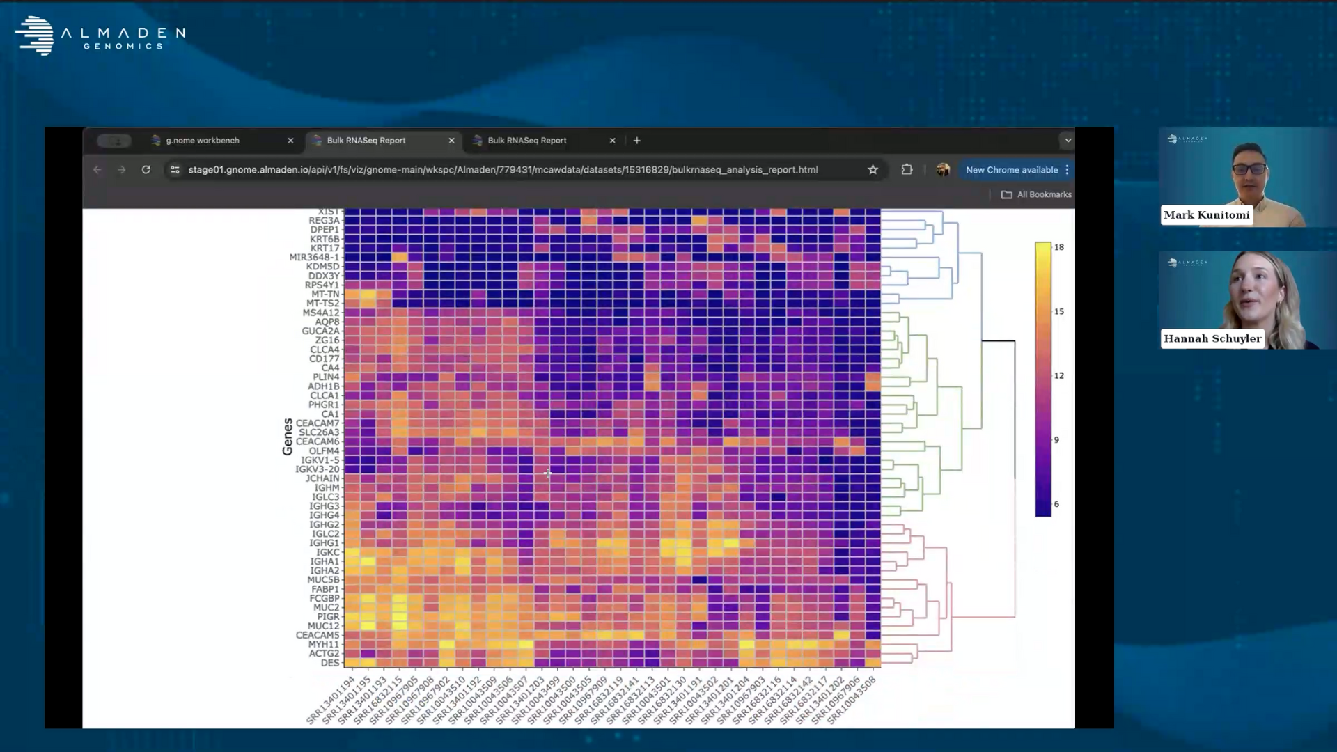
So the data is quite different, but all of the data is of high quality and I think that's really important to take a look at. The next thing that I'm going to want to take a look at is to go to our bulk RNA-seq report for differential expression. This is going to contain several different visualizations that are really key to being able to analyze this from a differential expression perspective.

We have made plots which are going to look at gene expression differences based on the amount of reads with a given gene. We have our PCA plots which are going to help us look at the similarity in differences between our samples and then volcano plots and heatmaps that are going to look at gene expression differences. The first thing to note that should be kind of a screaming red flag is when we look at our PCA, again, what this plot does is it takes the gene expression count data from each of those samples and reduces the dimensionality and to principal components so that you can have basically two dimensions to represent each sample and so you can represent each sample as a point on one of these plots. Its position is going to tell you it's relative similarity or difference from other samples within the dataset. Essentially the key takeaway from this type of plot is you want to see that samples that are from the same groups should be more similar to each other than they are to other groups.

For this type of experiment, what we might expect is that our normal tissues tend to be more similar to each other than our tumor tissues. But when we look at our PCA plot, that's not what we see at all. What we can see is that there's perhaps three different clusters that exist within the data, and each of those clusters here, here and here, contain a mix of both tumor and normal samples.

This is indicative of batch effects, which say something about the processing of the data, the person who did it, that kit that was used or the sequencer that was used in order to generate the data is contributing more technical variation than the samples themselves. If we take kind of a closer look at what the accession numbers are for this cluster down here, I don't expect to see it, but what I can tell you is that these are all accessions of similar numbers because they came from the same experiment. So lab coming from this data, from this sequence are from this person who processed it is more similar to itself than other datasets within our, our sample. And so we really need to be able to overcome this technical noise, otherwise it's going to lead to spurious comparisons for us identifying those downstream biomarkers.

We now know that our data is very heterogeneous, it's of high quality, but there's clearly some natural faults. How do we fix that? Luckily, g.nome contains a bunch of tooling that'll allow us to very rapidly perform that batch effect adjustment. We're going to come out of this front and we're going to go into our tool section. In addition to having our guided workflows on g.nome, we also have the ability to build your own workflows using our workflow builder. As I mentioned earlier, in order to do that, the first step is to bring in some tools so we can go to our tools section on that and then go to our add button in the top right and add tool.

So g.nome contains a library of open source tools. We have a few hundred different tools that are available. We're always adding new ones. I'm going to start by just searching for this tool, combat-seq, which is used to adjust for batch of facts. And I'm going to add it to our project. Now, when I do this, it's going to throw an error telling me that it's already been imported because I imported this previously, but that's basically the process of bringing it in. Now that we've done that, we're going to want to go over to our workflows and create a new workflow in order to bring together these tools as well as our data. I'm going to click on new workflow, call this batch correction, I already created one called batch correction when I'm not particularly creative, but from there that takes us to our workflow builder.

This is a graphical user interface that is a canvas where you can bring together our tooling as well as data and make visual connections instead of using code in order to perform an analysis. I'm going to bring in go to our module section and look for that combat-seq tool that I brought in. I'm going to bring in what we call a “tile” for that tool. And on that tile, we have the inputs on the left hand side, which consists of required inputs and optional inputs, and then our outputs on the right hand side.

What we can see from this combat-seq tool is that it has two required files which are going to be the counts file from our RNA-seq analysis and a batch file which I uploaded at the start of this webinar. So I'm going to go into data and I'm going to look for batch, bring that in. We're going to drag from what we call an outlook, which is on the right hand side of this file over to the inlet that says batch, and then I'm going to get my seq-counts file and drag that on and make that connection.

Now we have satisfied all of the input requirements in order to run this tool and I can drag and drop from the outlook side and create an output. This would create the output of this analysis, which is going to be a batch corrected change counts file so that I can do downstream analysis. Now the nice thing is that you don't have to run these as single tiles—you can make connections between them. What I'm going to do is I'm going to bring in an additional tile, which is a workflow for those visualizations that I want to be able to create. One of the things that it's going to take in is that adjusted count matrix. And then one of the other things that it's going to require are my sample metadata and a control name.

In order to do this, I'm going to go to my data. I upload previously my metadata for this study. I'll connect that over to the sample metadata. And then I'm also going to create a control name. A control name is a variable and this is going to be asking for a string I can drag out from that inlet and create a string object. From there, I'm just going to put in that I used the name normal for my control. After that, I'm going to drag out all the outputs that I want to generate from this analysis, and then I'm good to go from here. Since I have all of the connections made between these, I can now click run and give it a name.

And the same way in the guided workflow that this is launched in a cloud elastic nature. The same thing's going to happen for these runs and also save this workflow I want. I can also version it. We're going to call this 1.0.0. Now that job should be initiated in our runs tab. So of course I've already previously done this and we can come and take a look at the results from that.

What we can see when we now look at our bulk report, the PCA plot looks a lot more reasonable as we can see here. We really have two clusters of data, one which is our normal one, and one which is our tumor. We do have a little bit of overlap—oncology data is always going to be slightly messy, and so this data actually looks quite good from here.

We can also look at things like our MA plot and our MA plot is going to tell us what genes are differentially expressed and how highly are they expressed. We generally are going to want to see a nice mix of this. It's part of the quality control metric as well as gives us an indication of how much expression of these genes we're going to see.

Then we generate our standard heatmaps as well as volcano plots. One thing that I think is really of interest here is that you can see immediately that one of our most highly differentially expressed genes from this is that GUCA2B gene that was identified in this paper. It turns out that the other gene that they were talking about KR31A is also on this plot, however, it is not one of the most differentially expressed genes. It is significantly differentially expressed, but not as large as some of these other genes. We also went through and hand verified for many of these genes what their relation might be to colorectal cancer. Many of them showed up as having evidence that they're involved in colorectal cancer diagnosis or prognosis.

In fact, we identified, if you can look at the white paper that we have up on our website, a new gene that was recently identified as being associated with colorectal cancer. And so really this is the start for our users to be able to look at these differentially expressed genes, start to form hypotheses and experimental validation.

The last thing I'll say is for these outputs, in addition to having just the differential expression of reports, we also do gene set enrichment where you're going to get a bunch of different plots looking at different pathways or gene sets that are up or down regulated as part of this process and our pathway analysis. All of these, again, are that starting point for further downstream validation that you can use.

In addition to the plots that are generated automatically with our pipelines, we also have the ability to launch Jupyter notebooks so you can do further interactive analyses in order to explore your data.

That's going to do it for our live demo of g.nome today. What we did is really take you through the process of identifying a data that you want to be able to analyze, bringing in accessions and metadata, launching several workflows that allow you to bring in tens to hundreds of gigs of data that's publicly available in a very rapid process, analyze the data quite rapidly using our guided workflows, check on the quality of that data, and then be able to iterate based on what you find, i.e. to see that some of this data, although it's a high quality, it needs batch correction, then to perform that additional analysis and then come back to your results. I think that's really a key to exploring your data.

What g.nome does is allows you to get to these types of analyses in these types of iterations without all of the intervening pieces that are so frustrating and trying to run analyses on the cloud, trying to manage all of your data, trying to get individual tooling to install all correctly, to trying to get your cloud ability to scale to the data that you want to analyze.

g.nome removes all of those processes and really allows you to just focus on the data, its quality and its interpretations. With that, I'm going to stop then, and I'd love to take any questions that you may have.

Hannah Schuyler:

Thank you, Mark. And that was great. We've had a few questions come through, but again, feel free to type any additional questions in the chat box.

The first one, this was related to when you were doing the SRA pulling of the public data set. There's a question asking, does matter if the data is paired or not?

Mark Kunitomi:

We support the ability to bring in both paired and an unpaired data. And in fact, for single cell, you can also bring in data that is both paired plus has additional technical replicates. So yeah, this has the ability to do single end, paired end and even more exotic analyses.

Hannah Schuyler:

Great. This question says I am new to bioinformatics. What kind of support and resources are available for users of the g.nome platform?

For all of our workflows we have documentation. We also have training videos and we do onboarding to get you up to speed on how to use the software and then there's as much handholding support as you need. So depending on your comfort with using the software, we have customized training schedules and training plans for you, it's definitely flexible.

Mark Kunitomi:

We have a lot of biologists turned bioinformaticians who helped develop this platform. So we recognize, you know, the struggles that we've had as biologists trying to figure out these processes. And, you know, we try to make all the resources available as much as possible, but we're also that make sure that you have a successful experience on g.nome.

Hannah Schuyler:

Okay. We have one around the types of data analysis. Can g.nome be used for other types of omics data? And if so, what other applications?

Mark Kunitomi:

Absolutely. So in addition to being able to do bulk transcriptomic analysis or RNA-seq analysis, we also have things for looking at the DNA side of the house, so looking at variant calling and those types of analyses. We also have epigenetic analysis, use those things for ATAC-seq, methyl-seq, amongst a few others, and then we have single cell analysis that are on platform for single cell RNA-seq.

In addition to that, we also have the idea of tooling so you can build workflows in order to perform custom analysis. Really, our system is flexible enough to handle pretty much any data type and any non-streaming tooling. And so if you needs to build something yourself, that's something you can do or we can assist you in building in and custom workflow.

Hannah Schuyler:

Great. And then there's a follow up question around hands-on training, if there's any hands on training available. Yes, there is, we would be happy to support you in your analysis training. So we can send you a follow up note and connect on what that will look like.

There's a few more questions coming through. Is there any other option for alignment in addition to using STAR?

Mark Kunitomi:

Yeah. We have a bunch of different aligners that are on platform and so you can modify the workflow in order to use your favorite aligner, so that's certainly a possibility.

Hannah Schuyler:

How does that platform handle large datasets? Are there any limitations on the size of the data that we can upload and analyze?

Mark Kunitomi:

This is where a lot of back end engineering has come in. I can't claim that I understand every piece of it, but g.nome is incredibly scalable in terms of the size limits for data sets. Really, I would say there aren't datasets that that break us terms of scale. So there aren't datasets large enough that we've observed breaking for these types of workflows. So really, you can use incredibly large datasets on g.nome without having to worry about it.

Hannah Schuyler:

How can I customize the analysis parameters in g.nome for specific research needs?

Mark Kunitomi:

So there's a variety of ways that that can be done. And, you know, variety of kind of levels that guided workflow have. We have our advanced parameters, and so this is really for when you're tuning the workflow, you get to choose, you know, from a preset amount of different pathways within that. So for certain workflows, you can choose your aligner or certain ones, you can choose your read count methods. You also can do the small tweaking like you know how you want to you what values you want to use for p values or these types of things. So that's the kind of customization you can do within the guided workflow.

Within the workflow builder itself, the customization increases quite a bit because now you can take any of our modular tools and rewire them, bring in new tooling, remove parts of the analysis, add parts of the analysis so you can change not only the parameters that exist for all of those tools, but you can change the wiring itself or the tooling that's used itself. So it's incredibly customizable.

Hannah Schuyler:

Okay. We have a question around pathways that is, are databases for gene ontology and pathways updated automatically or sent by the user? And can users use other databases for functional analysis like React or Wiki pathways.

Mark Kunitomi:

We have been updating our pathways for pathway analysis. Bringing in custom pathways is something that can be done. I think we can make that easier to do in the future, to be honest. But yes, absolutely, you can bring them in.

Hannah Schuyler:

One last question. What are the pre-processing steps that are done for RNA-seq quality control?

Mark Kunitomi:

A lot of the bulk of what gets done is using fastp, which is a combination of a couple of tools that looks a read trimming based on quality and then adapter removal. But there's a lot of different flavors that you can use depending on which pipeline or what parameters that you use. For some, you can also remove things like ribosomal RNA, you can those things can be filtered out, but the bulk of it is done in terms of adapter removal and then sequence quality.

Hannah Schuyler:

Awesome. I think that wraps our questions for now. Thank you again, Mark, for your time, and everyone for joining.